Is the gradient of an algorithm the gradient of the solution?
Two functions under the same notation
In the dissertation I am working on, the gradient passes through a fixed number of solver steps during training; at inference, the solver uses stopping criteria. This difference got me thinking:
What are we learning when we differentiate a truncated optimization process?
A network layer can be defined by an optimization problem. The input determines a cost function, and the solution to that problem is passed to the rest of the model. In code, this computation usually takes the form of a loop of solver updates. We can then backpropagate the loss gradient through these updates to train the model.
The algorithm, however, returns the result of a finite number of steps. Automatic differentiation acts on this finite computation. For the resulting gradient to match that of the problem’s solution, we need additional conditions. The difference can be large enough for the two gradients to have opposite signs.
I want to follow this difference from the chain rule to an example that fits in a few lines of code — there is no need for a deep network: a strictly convex quadratic with two variables and an explicit solution is enough to separate the effects.
Let \(z\in\mathbb{R}^d\) be the inner variable and \(\theta\in\mathbb{R}^p\) the parameters we want to learn. I write the solution to the inner problem as
\[ z^\star(\theta)=\operatorname*{arg\,min}_{z} f(z,\theta). \]
An outer loss \(\ell\) evaluates this solution. For example, \(f\) might combine data fidelity and regularization, while \(\ell\) measures the error of a prediction obtained from \(z\). The function we would like to minimize is
\[ L_\star(\theta)=\ell(z^\star(\theta),\theta). \]
For now, I assume that the minimum is unique and that the derivatives used below exist. These assumptions will need to be made more precise later.
In the implementation, we choose an initialization \(z_0(\theta)\), an update \(T\), and a budget of \(K\) steps:
\[ z_{k+1}(\theta)=T(z_k(\theta),\theta), \qquad L_K(\theta)=\ell(z_K(\theta),\theta). \]
The composition of \(K\) updates defines another function of the parameters. The initialization, step size, and number of iterations are part of its definition. If all dependencies are preserved in the graph, automatic differentiation computes \(\nabla_\theta L_K\), subject to the numerical errors of the arithmetic used.1
Training this composition can be a deliberate choice. Domke studies precisely this setting: models trained using the output of an optimization procedure truncated after a fixed number of iterations.2 For an application that will also execute only those steps, \(L_K\) may be the objective of interest. The issue arises when we write \(L_\star\) in the formulation and interpret the gradient of \(L_K\) as though the substitution were harmless.
Differentiating the steps
Sensitivity also follows a recurrence
Define the sensitivity matrix
\[ J_k=\frac{\partial z_k}{\partial\theta} \in\mathbb{R}^{d\times p}. \]
Applying the chain rule to the update gives
\[ J_{k+1} = D_zT(z_k,\theta)J_k + D_\theta T(z_k,\theta). \]
The first term carries forward the dependence accumulated in previous steps. The second captures the current update’s direct dependence on \(\theta\). For a constant initialization, \(J_0=0\). If the initialization is the output of another network, its derivative must enter as \(J_0\).
After \(K\) steps, the loss derivative is
\[ \nabla_\theta L_K = \nabla_\theta\ell(z_K,\theta) + J_K^\top\nabla_z\ell(z_K,\theta), \]
where the first term is a partial derivative: \(z_K\) is held fixed when computing it. This expression makes explicit what automatic differentiation needs to propagate.
Constructing \(J_k\) explicitly is convenient for the derivation and for examples with few parameters. When \(\theta\) has millions of components and the loss is scalar, reverse mode computes the required products without materializing the entire matrix. Both modes apply the same chain rule to the same function. Franceschi and colleagues develop these two ways of propagating derivatives through iterative learning algorithms, with different time and memory costs.3
The gradient descent case
Consider a fixed step size \(\eta\), independent of \(\theta\):
\[ z_{k+1}=z_k-\eta\nabla_z f(z_k,\theta). \]
With
\[ H_k=\nabla^2_{zz}f(z_k,\theta), \qquad B_k=(D_\theta\nabla_z f)(z_k,\theta), \]
where the partial derivative defining \(B_k\) holds \(z\) fixed and is then evaluated at \((z_k,\theta)\), we obtain
\[ J_{k+1}=(I-\eta H_k)J_k-\eta B_k. \]
Differentiating through an update that already uses a gradient therefore introduces second-order derivatives. We do not need to build a dense Hessian to do this: Hessian–vector products may suffice. Pearlmutter gives a way to compute them without storing the full matrix.4 Removing these dependencies from the graph changes the derivative being computed.
We also need to distinguish two forms of truncation. Executing \(K\) steps and differentiating through all of them produces \(\nabla_\theta L_K\). Executing many steps, cutting off the history with detach, and backpropagating only through the final steps treats the state at the cut as constant. In the second case, the derivative of the original computation has been modified. Shaban and colleagues study the approximate gradients produced by this truncation and give sufficient conditions for convergence of the outer optimization.5
Differentiating the solution
The optimality condition
For an unconstrained problem, an interior solution satisfies
\[ \nabla_z f(z^\star(\theta),\theta)=0. \]
Suppose that \(f\) is twice continuously differentiable in a neighborhood of the solution and that
\[ H_\star=\nabla^2_{zz}f(z^\star,\theta) \]
is invertible. The implicit function theorem lets us locally track this stationary point as a differentiable function of \(\theta\). A positive definite Hessian ensures that the branch being tracked continues to consist of local minima; global strong convexity, when present, also ensures uniqueness of the minimum. For nonconvex problems, the analysis is local and does not resolve possible switches between minima.
Differentiating the optimality condition,
\[ H_\star J_\star+B_\star=0, \qquad J_\star=-H_\star^{-1}B_\star, \]
where \(J_\star=\partial z^\star/\partial\theta\) and \(B_\star=(D_\theta\nabla_z f)(z^\star,\theta)\).
The optimizer’s update has disappeared from the expression. The derivative depends on the geometry of the problem at the chosen minimum. Two algorithms that find the same regular solution yield the same implicit sensitivity, even if they follow different trajectories. Blondel and colleagues explore this separation between the solver and the equation defining its derivative.6
The adjoint system
Substituting \(J_\star\) into the chain rule,
\[ \nabla_\theta L_\star = \nabla_\theta\ell(z^\star,\theta) - B_\star^\top H_\star^{-\top}\nabla_z\ell(z^\star,\theta). \]
The inverse helps us read the formula, but it is not an instruction to compute it. We only need to solve
\[ H_\star^\top v=\nabla_z\ell(z^\star,\theta) \]
and then use
\[ \nabla_\theta L_\star = \nabla_\theta\ell(z^\star,\theta)-B_\star^\top v. \]
This is the adjoint system. It avoids constructing a \(d\times p\) Jacobian when we only need the derivative of a scalar loss.
It is tempting to dismiss this calculation by saying that the inner gradient is zero at the minimum. That argument applies, for example, when the outer function is the optimal value of \(f\) itself. Indeed,
\[ \nabla_\theta\bigl[f(z^\star(\theta),\theta)\bigr] = \nabla_\theta f(z^\star,\theta) + J_\star^\top \underbrace{\nabla_z f(z^\star,\theta)}_{0}. \]
This identity is the smooth, unconstrained case of the envelope argument. For a different outer loss, \(\nabla_z\ell(z^\star,\theta)\) is generally nonzero. The fact that \(z^\star\) minimizes \(f\) does not justify ignoring how it varies inside \(\ell\).
When the derivatives approach each other
The two constructions meet when the update converges to the solution and its sensitivity also converges. If \(z^\star=T(z^\star,\theta)\), differentiating this equation gives
\[ \bigl(I-D_zT(z^\star,\theta)\bigr)J_\star = D_\theta T(z^\star,\theta). \]
The same calculation appears in the deep equilibrium models of Bai, Kolter, and Koltun: the state is defined as a fixed point, found by a root solver, and backpropagation uses implicit differentiation.7 The equilibrium equation can define the layer even when the update does not correspond to a minimization step.
When the spectral radius of \(D_zT(z^\star,\theta)\) is less than one, the inverse can be written as a Neumann series:
\[ J_\star = \sum_{i=0}^{\infty} \bigl[D_zT(z^\star,\theta)\bigr]^i D_\theta T(z^\star,\theta). \]
This series uses the Jacobians evaluated at the fixed point. Along a nonlinear trajectory, the Jacobians change at each step; finite unrolling is generally not just a truncation of this same series.
I will use the Euclidean norm for vectors and the corresponding operator norm for matrices. A stronger sufficient condition, useful for understanding convergence, is that \(T\) be a uniform contraction on a region containing the trajectory and the fixed point, for parameters in a neighborhood of the point under study, with a factor \(0<q<1\). Assume also that \(T\) is continuously differentiable and that its partial derivatives are Lipschitz in \(z\) on that region. With \(\theta\) fixed, the sensitivity recurrence gives the error bound
\[ \|J_{k+1}-J_\star\| \leq q\|J_k-J_\star\|+c\|z_k-z^\star\|, \]
for a constant \(c\) that depends on these derivatives and on \(J_\star\). Since the contraction also gives \(\|z_k-z^\star\|\leq Dq^k\), with \(D=\|z_0-z^\star\|\), it follows that
\[ \|J_K-J_\star\| \leq q^K\|J_0-J_\star\| + cD Kq^{K-1}. \]
Both terms tend to zero. With continuous derivatives of the outer loss, we also obtain \(\nabla_\theta L_K\to\nabla_\theta L_\star\). Grazzi and colleagues provide quantitative bounds on these errors under contraction and regularity assumptions.8
These assumptions matter. Convergence of the values of a sequence of functions alone does not justify exchanging differentiation and the limit. Even when everything converges, a \(q\) close to one can require many steps to obtain a good approximation of the sensitivity.
A quadratic with two scales
Closed-form solution and trajectory
Now consider a scalar parameter \(\theta\) and the problem
\[ f(z,\theta)=\frac12z^\top Az-\theta b^\top z, \qquad A= \begin{pmatrix} 1&0\\ 0&0.01 \end{pmatrix}, \qquad b= \begin{pmatrix} 1\\ 0.01 \end{pmatrix}. \]
Since \(A\) is positive definite, the minimum is unique:
\[ Az^\star=\theta b \quad\Longrightarrow\quad z^\star(\theta)=\theta A^{-1}b = \begin{pmatrix} \theta\\ \theta \end{pmatrix}. \]
I choose the outer loss
\[ \ell(z)=\frac12\|z-y\|_2^2, \qquad y= \begin{pmatrix} 0\\ 3 \end{pmatrix}. \]
Then,
\[ L_\star(\theta)=\frac12\bigl[\theta^2+(\theta-3)^2\bigr], \qquad g_\star(\theta)=\frac{dL_\star}{d\theta}=2\theta-3. \]
At \(\theta=1\), the derivative is \(g_\star=-1\). A small increase in \(\theta\) reduces the outer loss evaluated at the solution.
Gradient descent, in turn, follows
\[ z_{k+1}=(I-\eta A)z_k+\eta\theta b. \]
Define \(M=I-\eta A\). For a constant initialization, summing the matrix geometric progression gives
\[ z_K=M^Kz_0+\theta(I-M^K)A^{-1}b, \]
and therefore
\[ J_K=(I-M^K)A^{-1}b, \qquad J_\star=A^{-1}b. \]
Here, the connection between unrolling and the Neumann series is exact:
\[ J_K=\eta\sum_{i=0}^{K-1}M^i b. \]
For \(0<\eta<2/\lambda_{\max}(A)\), all eigenvalues of \(M\) have magnitude less than one. Thus, \(M^K\to0\) and \(J_K\to J_\star\). In a direction with curvature \(\lambda\), the sensitivity is multiplied by the factor
\[ 1-(1-\eta\lambda)^K. \]
The direction with small curvature can take a long time to acquire its full sensitivity.
A gradient with the opposite sign
Use \(\eta=1\), \(z_0=(0,0)^\top\), and evaluate at \(\theta=1\). For \(K\geq1\), writing \(q_K=0.99^K\),
\[ z_K= \begin{pmatrix} 1\\ 1-q_K \end{pmatrix}, \qquad J_K= \begin{pmatrix} 1\\ 1-q_K \end{pmatrix}. \]
The unrolled gradient is
\[ \begin{aligned} g_K &=(z_K-y)^\top J_K\\ &=1+(-2-q_K)(1-q_K)\\ &=-1+q_K+q_K^2. \end{aligned} \]
The distance to the solution and the inner objective gap are
\[ \|z_K-z^\star\|_2=q_K, \qquad f(z_K,1)-f(z^\star,1)=0.005q_K^2. \]
After 40 steps, \(q_K\approx0.6690\). The inner objective gap is about \(0.00224\), but the error in the solution is still \(0.6690\). The low curvature in the second coordinate makes this error relatively inexpensive for \(f\). There is no reason for it to be inexpensive for \(\ell\) as well.
At this point,
\[ g_{40}\approx+0.1165, \qquad g_\star=-1. \]
An outer update \(\theta\leftarrow\theta-\alpha g_{40}\), with a small \(\alpha>0\), decreases \(\theta\). It is a descent direction for \(L_{40}\), but an ascent direction for \(L_\star\) at that point. The differentiation is correct for the function that was executed.
What if the algorithm already returns the exact solution?
It is worth making one change to the example. Now fix the initialization at \(z_0=(1,1)^\top\), keeping this same vector for all values of \(\theta\). At the evaluation point \(\theta=1\), the initialization coincides with the minimum, and the updates do not move the state:
\[ z_K(1)=z^\star(1) \qquad\text{for all }K. \]
Even so, because the initialization is constant, \(J_0=0\). The sensitivity after \(K\geq1\) steps is still \((1,1-q_K)^\top\). Now,
\[ g_K=(1,-2) \begin{pmatrix} 1\\ 1-q_K \end{pmatrix} =-1+2q_K. \]
For \(K=40\), this gives \(g_K\approx+0.3379\). The state is exactly at the minimum, the optimality residual is zero, and the derivative still has the opposite sign to \(g_\star\).
The example was constructed so that the two functions agree at one point. When \(\theta\) is perturbed, the initial vector remains at \((1,1)^\top\), while the solution moves to \((\theta,\theta)^\top\). The two functions meet at \(\theta=1\), but have different tangents.
Had we defined a differentiable initialization \(z_0(\theta)=(\theta,\theta)^\top\), then \(J_0=(1,1)^\top\), and the derivative would have been correct from the start. This distinction also arises when reusing a previous solution as a warm start: holding it constant during differentiation is a choice about the dependence the program will represent.
Implementing the example
The NumPy code computes the trajectory, propagates its sensitivity, and compares the derivatives with finite differences.
Derivatives and finite differences
The run_steps function propagates sensitivity in forward mode. It writes out the chain rule explicitly, making it possible to follow the dependence on the initialization and the number of steps. The central difference evaluates the same computation at two nearby parameter values.
from collections.abc import Callable

import numpy as np

a = np.array([1.0, 0.01], dtype=np.float64)  # diagonal of A
b = np.array([1.0, 0.01], dtype=np.float64)
y = np.array([0.0, 3.0], dtype=np.float64)


def run_steps(
    theta: float, k: int, z0: np.ndarray, eta: float = 1.0
) -> tuple[np.ndarray, np.ndarray]:
    """Return z_K and dz_K/dtheta, keeping z0 constant."""
    z = np.array(z0, dtype=np.float64, copy=True)
    j = np.zeros_like(z)
    for _ in range(k):
        z = z - eta * (a * z - theta * b)
        j = (1.0 - eta * a) * j + eta * b
    return z, j


def loss(z: np.ndarray) -> float:
    """Quadratic outer loss."""
    return float(0.5 * np.dot(z - y, z - y))


def central_difference(
    function: Callable[[float], float], theta: float, h: float
) -> float:
    return (function(theta + h) - function(theta - h)) / (2.0 * h)


theta, k, h = 1.0, 40, 1e-5
for z0 in (np.zeros(2), np.ones(2)):
    z, j = run_steps(theta, k, z0)
    g = float((z - y) @ j)
    fd = central_difference(
        lambda t: loss(run_steps(t, k, z0)[0]), theta, h
    )
    print(f"z0={z0}: chain rule={g:+.9f}; finite differences={fd:+.9f}")

z_star = np.linalg.solve(np.diag(a), theta * b)
v = np.linalg.solve(np.diag(a).T, z_star - y)
g_star = float(b @ v)  # B = -b; hence -B^T v = b^T v
fd_star = central_difference(lambda t: loss(t * b / a), theta, h)
print(f"implicit={g_star:+.9f}; finite differences={fd_star:+.9f}")

# z0=[0. 0.]: chain rule=+0.116494972; finite differences=+0.116494972
# z0=[1. 1.]: chain rule=+0.337943517; finite differences=+0.337943517
# implicit=-1.000000000; finite differences=-1.000000000
Varying the number of steps
The same function lets us compare the two initializations for different numbers of steps. The block below computes the gradients and, for the zero initialization, the distance to the solution and the inner objective gap.
print("   K     state error   inner gap     g_K (zero)   g_K (constant)")
for k in (1, 10, 40, 100, 400, 1000):
    z, j = run_steps(1.0, k, np.zeros(2))
    z_const, j_const = run_steps(1.0, k, np.ones(2))
    error = z - b / a
    # The quadratic identity avoids subtracting nearly equal objective values.
    gap = float(0.5 * np.dot(a * error, error))
    g = float((z - y) @ j)
    g_const = float((z_const - y) @ j_const)
    print(
        f"{k:4d}   {np.linalg.norm(error):.6f}   {gap:.3e}"
        f"      {g:+.6f}     {g_const:+.6f}"
    )
The table shows the rounded results. The error and objective gap columns correspond to the zero initialization.
| \(K\) | Solution error | Inner objective gap | \(g_K\), start at \((0,0)\) | \(g_K\), constant start at \((1,1)\) |
|---|---|---|---|---|
| 1 | 0.990000 | \(4.901\times10^{-3}\) | +0.970100 | +0.980000 |
| 10 | 0.904382 | \(4.090\times10^{-3}\) | +0.722289 | +0.808764 |
| 40 | 0.668972 | \(2.238\times10^{-3}\) | +0.116495 | +0.337944 |
| 100 | 0.366032 | \(6.699\times10^{-4}\) | −0.499988 | −0.267935 |
| 400 | 0.017951 | \(1.611\times10^{-6}\) | −0.981727 | −0.964099 |
| 1000 | 0.000043 | \(9.319\times10^{-12}\) | −0.999957 | −0.999914 |
In every row, \(g_\star=-1\). For the constant initialization at \((1,1)\), the solution error and objective gap are zero at the evaluation point.
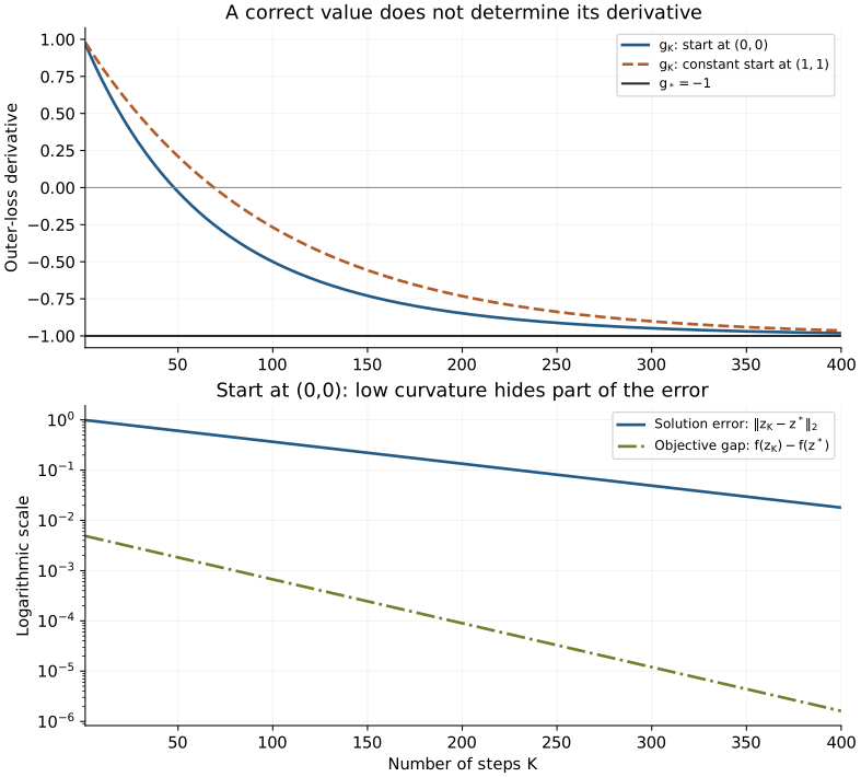
Top: outer-loss derivatives at θ = η = 1, compared with the derivative through the solution map. Bottom: state error and inner objective gap for the zero initialization, on a logarithmic scale. Values computed from the recurrences in the example.
What finite differences check
The central difference
\[ \frac{L_K(\theta+h)-L_K(\theta-h)}{2h} \]
checks the gradient of \(L_K\). Both evaluations must use the same \(K\), the same step size, and the same constant initialization. For the run initialized at \((1,1)^\top\), recomputing the initialization as \((\theta+h,\theta+h)^\top\) and \((\theta-h,\theta-h)^\top\) would change the function being tested.
To check \(g_\star\), we evaluate the solutions of the perturbed problems:
\[ \frac{L_\star(\theta+h)-L_\star(\theta-h)}{2h}. \]
In this example, those solutions are known in closed form. When that is not the case, the solver tolerance must be tight enough that evaluation errors do not dominate the division by \(h\).
State tolerance and derivative tolerance
Numerical implicit differentiation involves two approximations to control: the solution of the inner problem and the solution of the adjoint system.
For a differentiable, \(\mu\)-strongly convex objective, the stationarity residual bounds the state error:
\[ \|\widehat z-z^\star\| \leq \frac{\|\nabla_z f(\widehat z,\theta)\|}{\mu}. \]
This follows from strong monotonicity of the gradient,
\[ \bigl\langle \nabla_z f(\widehat z,\theta)-\nabla_z f(z^\star,\theta), \widehat z-z^\star \bigr\rangle \geq \mu\|\widehat z-z^\star\|^2, \]
combined with Cauchy–Schwarz and \(\nabla_z f(z^\star,\theta)=0\). A small residual must be interpreted in light of the minimum curvature \(\mu\).
Even if \(z^\star\) is exact, the adjoint system may be solved only approximately. If \(\widehat v\) has residual
\[ r_v=H_\star^\top\widehat v-\nabla_z\ell(z^\star,\theta), \]
then
\[ \widehat v-v=H_\star^{-\top}r_v. \]
For \(\widehat g=\nabla_\theta\ell-B_\star^\top\widehat v\), computed at that same exact point,
\[ \|\widehat g-\nabla_\theta L_\star\| \leq \|B_\star\|\,\|H_\star^{-\top}\|\,\|r_v\|. \]
The norm of the inverse can amplify the residual. If we also replace \(z^\star\) with \(\widehat z\), an additional error appears because the Hessian, mixed derivatives, and loss gradient are evaluated at a different point. Controlling it requires regularity and conditioning assumptions. Blondel and colleagues explicitly address the Jacobian error when the inner solution is approximate.6
Controlling these errors also affects the outer optimization. Pedregosa analyzes hyperparameter updates with inexact gradients and establishes convergence conditions that include regularity of the functions and summability of the errors.9 The accuracy required of each inner solve can therefore be part of the optimization method itself.
These residuals do not certify the unrolled gradient: the example initialized at \((1,1)\) already showed a zero inner residual and incomplete sensitivity. They serve a different purpose, concerning the approximation of the equations that define the implicit gradient.
There is also a difference between a loop with fixed \(K\) and one that stops upon reaching a tolerance. In the latter, the number of steps can change with \(\theta\). In a region where the stopping decisions remain unchanged, differentiating the executed path can be valid. At transitions between paths, the implemented function may cease to be differentiable. Finite-difference perturbations can also cross these transitions.
When there are constraints
The condition \(\nabla_z f=0\) must be replaced by the conditions appropriate to the problem. OptNet is a reference for constructing quadratic optimization layers and obtaining their derivatives from the Karush–Kuhn–Tucker, or KKT, conditions.10
One useful case is choosing weights that sum to one. Now \(w,\theta\in\mathbb{R}^d\). Consider a fixed matrix \(Q\succeq0\), a fixed scalar \(\tau>0\), and
\[ w^\star(\theta) = \operatorname*{arg\,min}_{w\in\Delta} \left\{ \frac12w^\top Qw-\theta^\top w +\tau\sum_i w_i\log w_i \right\}, \qquad \Delta=\{w\geq0:\mathbf1^\top w=1\}, \]
with the continuous extension \(0\log0=0\). For finite parameters, the entropy term guarantees a unique minimum in the relative interior of the simplex. At that point, the conditions are
\[ Qw-\theta+\tau(\log w+\mathbf1)+\lambda\mathbf1=0, \qquad \mathbf1^\top w=1. \]
The logarithm acts componentwise, and \(\lambda\) is the multiplier for the sum constraint. Defining
\[ H=Q+\tau\operatorname{diag}(1/w_i), \]
differentiation gives
\[ \begin{pmatrix} H&\mathbf1\\ \mathbf1^\top&0 \end{pmatrix} \begin{pmatrix} dw\\ d\lambda \end{pmatrix} = \begin{pmatrix} d\theta\\ 0 \end{pmatrix}. \]
The second row imposes \(\mathbf1^\top dw=0\): the sensitivities remain in the tangent space of the simplex. Solving a system with \(H\) alone would ignore this constraint. In this example, \(H\) is positive definite and the equality constraint has full rank, making the block system invertible.
More care is needed when inequality constraints become active or inactive. Even a strongly convex objective can define a nondifferentiable solution map:
\[ \operatorname*{arg\,min}_{z\geq0}\frac12(z-\theta)^2 = \max(0,\theta). \]
The minimum is unique for every \(\theta\), but its derivative does not exist at zero. Uniqueness of the solution is therefore not enough to apply a smooth formula through every change in the active set.
Which function will be used after training?
For a layer that will execute exactly \(K\) steps, I find it natural to start with \(L_K\). The budget is part of the model, and training can learn to make use of it. Increasing the number of steps afterward changes the function being evaluated; improving the inner objective does not guarantee an improvement in the outer loss. This possibility is one reason to treat truncated optimization as an explicit definition of the model.2
When the solution to the problem is what matters, implicit differentiation allows the solver to be chosen on numerical grounds. In return, we need to solve the inner problem to adequate accuracy and check the adjoint system. In a typical implementation, reverse mode through \(K\) steps stores intermediate states; checkpointing trades some of that memory for recomputation. The implicit method avoids storing this trajectory for the derivative calculation, but adds a linear system whose cost depends on conditioning and on the products we can compute.8 Neither approach has a universal runtime advantage.
Before comparing methods, I would start the diagnosis with the outer function: write down \(L_K\) or \(L_\star\), fix the initialization rule, and check each derivative against perturbations of that same function. I would then vary the budget and tolerances to observe the state error and gradient error separately. In the example, keeping them separate was enough to understand why three correct numbers, \(+0.1165\), \(+0.3379\), and \(-1\), describe such different behavior.
References
-
BAYDIN, A. G.; PEARLMUTTER, B. A.; RADUL, A. A.; SISKIND, J. M. Automatic differentiation in machine learning: a survey. Journal of Machine Learning Research, vol. 18, no. 153, pp. 1–43, 2018. ↩
-
DOMKE, J. Generic methods for optimization-based modeling. In: Proceedings of the Fifteenth International Conference on Artificial Intelligence and Statistics. PMLR, vol. 22, pp. 318–326, 2012. ↩ ↩2
-
FRANCESCHI, L.; DONINI, M.; FRASCONI, P.; PONTIL, M. Forward and reverse gradient-based hyperparameter optimization. In: Proceedings of the 34th International Conference on Machine Learning. PMLR, vol. 70, pp. 1165–1173, 2017. ↩
-
PEARLMUTTER, B. A. Fast exact multiplication by the Hessian. Neural Computation, vol. 6, no. 1, pp. 147–160, 1994. ↩
-
SHABAN, A.; CHENG, C.-A.; HATCH, N.; BOOTS, B. Truncated back-propagation for bilevel optimization. In: Proceedings of the Twenty-Second International Conference on Artificial Intelligence and Statistics. PMLR, vol. 89, pp. 1723–1732, 2019. ↩
-
BLONDEL, M.; BERTHET, Q.; CUTURI, M.; FROSTIG, R.; HOYER, S.; LLINARES-LÓPEZ, F.; PEDREGOSA, F.; VERT, J.-P. Efficient and modular implicit differentiation. In: Advances in Neural Information Processing Systems, vol. 35, 2022. ↩ ↩2
-
BAI, S.; KOLTER, J. Z.; KOLTUN, V. Deep equilibrium models. In: Advances in Neural Information Processing Systems, vol. 32, 2019. ↩
-
GRAZZI, R.; FRANCESCHI, L.; PONTIL, M.; SALZO, S. On the iteration complexity of hypergradient computation. In: Proceedings of the 37th International Conference on Machine Learning. PMLR, vol. 119, pp. 3748–3758, 2020. ↩ ↩2
-
PEDREGOSA, F. Hyperparameter optimization with approximate gradient. In: Proceedings of the 33rd International Conference on Machine Learning. PMLR, vol. 48, pp. 737–746, 2016. ↩
-
AMOS, B.; KOLTER, J. Z. OptNet: differentiable optimization as a layer in neural networks. In: Proceedings of the 34th International Conference on Machine Learning. PMLR, vol. 70, pp. 136–145, 2017. ↩